Both the gridding and CLEAN kernels were parallelized by pixel (in the uv and image plane respectively). The latter greatly benefited from this choice since once the maxima has been located in the dirty image the convolution is embarassingly parralel for both building the CLEANed image and subracting from the dirty image. For each iteration we call pyCUDA's max() function and used atomic operations to locate the peak's position in the image. The speed of this kernel and the quality of our CLEANed images might be improved by including a masking option that would limit the search area. One might also be able to combine the max() and locate() steps into one kernel optimized for the square grids we generate. Additionally, we build up the CLEANed image during the CLEAN iterations. This is faster than constructing the image at the end through multiple convolutions. However we coule implement this step using an FFT and multiplication. This might result in a factor of ~2 improvement in speedup. We tried a few advanced optimizations using texture memory and meta-programming with Cheetah but saw little measurable improvement.

Our implementation of the gridding kernel is much more expensive than the FFT, weighting, and shifting kernels (for our test datasets). The large number of visibilities (~1.5 million for the Fomalhaut dataset) that must be moved onto the GPU makes memory a limiting factor. Performance improved greatly (speedups of ~10) by leveraging the Hermitian nature of the data and the minimum baseline to reduce the gridding region. We also averaged the data in various ways to reduce the size of the datasets and removed flagged visibilities on the CPU. We keep the convolution kernel in constant memory and tried various optimization schemes such as shared and staggered memory access. Better performance might be achieved by pre-processing (e.g. sorting and indexing) the data on the CPU (see this report)).

Imaging spectral image cubes or multi-frequency synthesis would benefit by parallelizing this application using MPI across multiple GPUs. Additionally, extending this application to more advanced versions of the CLEAN algorithm is possible and might benefit from the speedups we report. Lastly, our kernels and python code provide a framework that can be extended for analyzing complex visibilities on the GPU.

Here are timings output by our GPU code for the source ϵ Mouse :

Gridding execution time 2.12 0.06s
        0.0000096 s per visibility
  Hogbom execution time 3.270.02 s
        0.0013 s per iteration

A reference implementation of the Hogbom algorithm in numpy took:

Serial execution time 251.6380  s
         0.0908  s per iteration 

The standard radio astronomy software CASA took 14.40.07 s for both gridding and CLEANing.

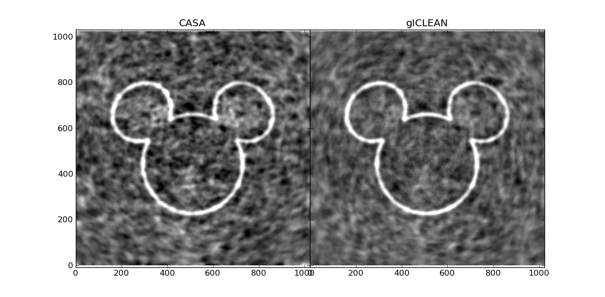
We therefore achieve a Hogbom speedup of 70x compared to the reference numpy implementation, which is an identical CLEAN algorithm. Our routine has a 2.7x speedup compared to the CASA implementation, which apparently is already significantly optimized compared to the reference implementation. The final CLEANed images from our implementation and CASA are compared below:

The execution time per visibility is independent of the source’s structure but does scale with the number of samples as well as the sampling coverage. The time per Hogbom iteration should be independent of all characteristics except image dimensions. Indeed, with we find similar timings with all our examples using 1024x1024 image dimensions. Increasing the image dimensions, we find that the gridding execution time remains approximately the same, while the Hogbom execution time grows approximately linearly with the number of pixels.

• A description of the Hogbom algorithm by the National Radio Astronomy Observatory:
  http://www.cv.nrao.edu/~abridle/deconvol/node8.html
• Hogbom’s original 1974 paper
• The radio astronomy data reduction packages CASA and MIRIAD
• A reference implementation of the Hogbom algorithm in numpy

Finally, note that the following is printed at the end of each run of the code:

Exception scikits.cuda.cufft.cufftInvalidPlan: cufftInvalidPlan() in > ignored

This exception does not seem to affect the execution of the code in any way.