The input data are complex valued and must be gridded (this example is an offset, inclined ring):

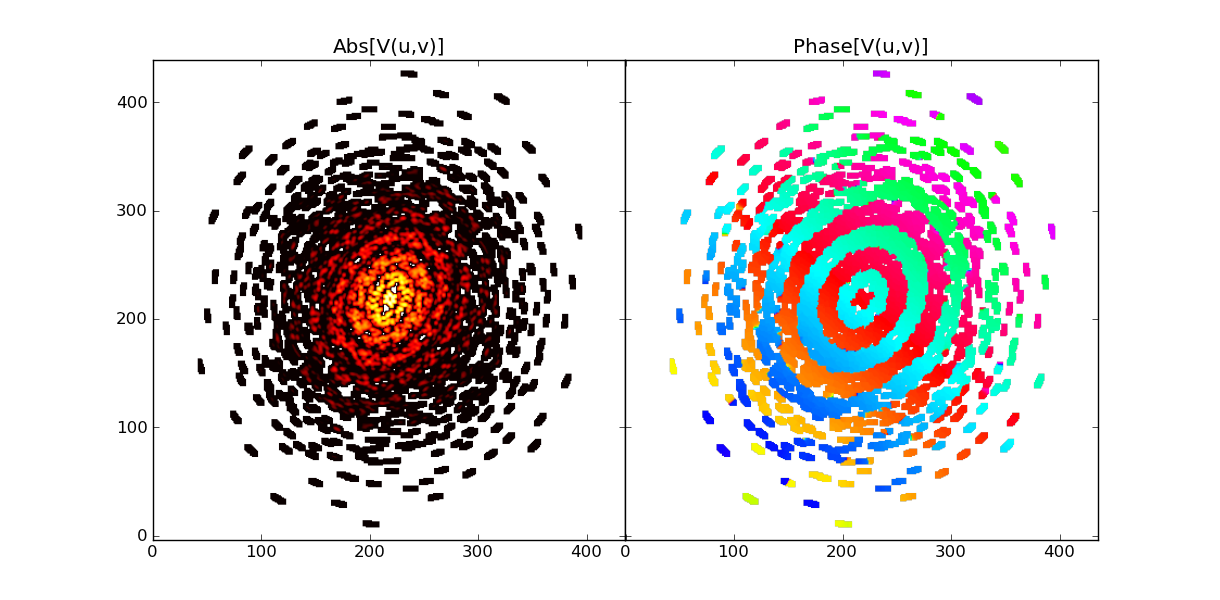
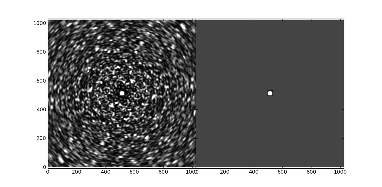
The sampling pattern in the complex plane determines the shape of the dirty beam shown below (left) and is approximated by a clean beam (right), which preserves only the primary lobe.

The Hogbom algorithm iteratively finds the pixel with maximum absolute intensity on the dirty image and subtracts the dirty beam shifted and scaled to that location/intensity. Below we show a simulated dirty image of the fictional astrophysical sources ϵ Mouse (left) and the first three iterations of the dirty beam subtraction (right).

Click on this image to see an animated version.

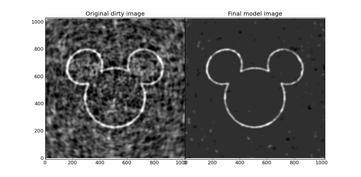
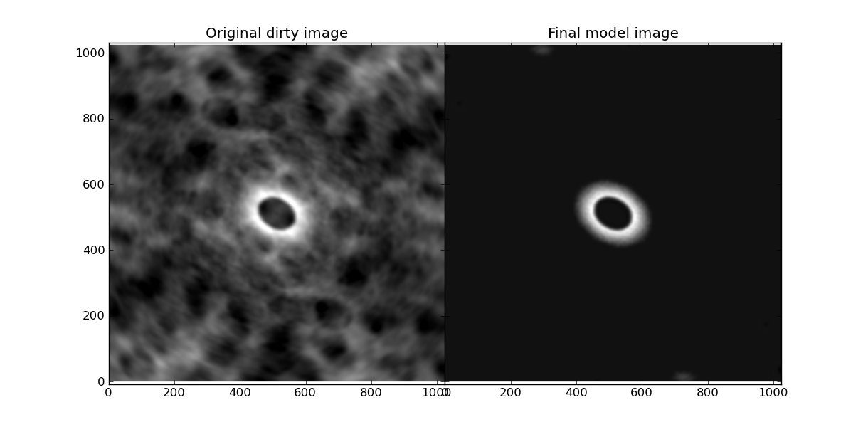
The Hogbom algorithm converges to within the specified threshold (0.2 times the initial maximum intensity, in this case) after 2700 iterations. At each iteration, it has added a point source to its model for the image, shown below at right. The model closely resembles the astrophysical source ϵ Mouse:

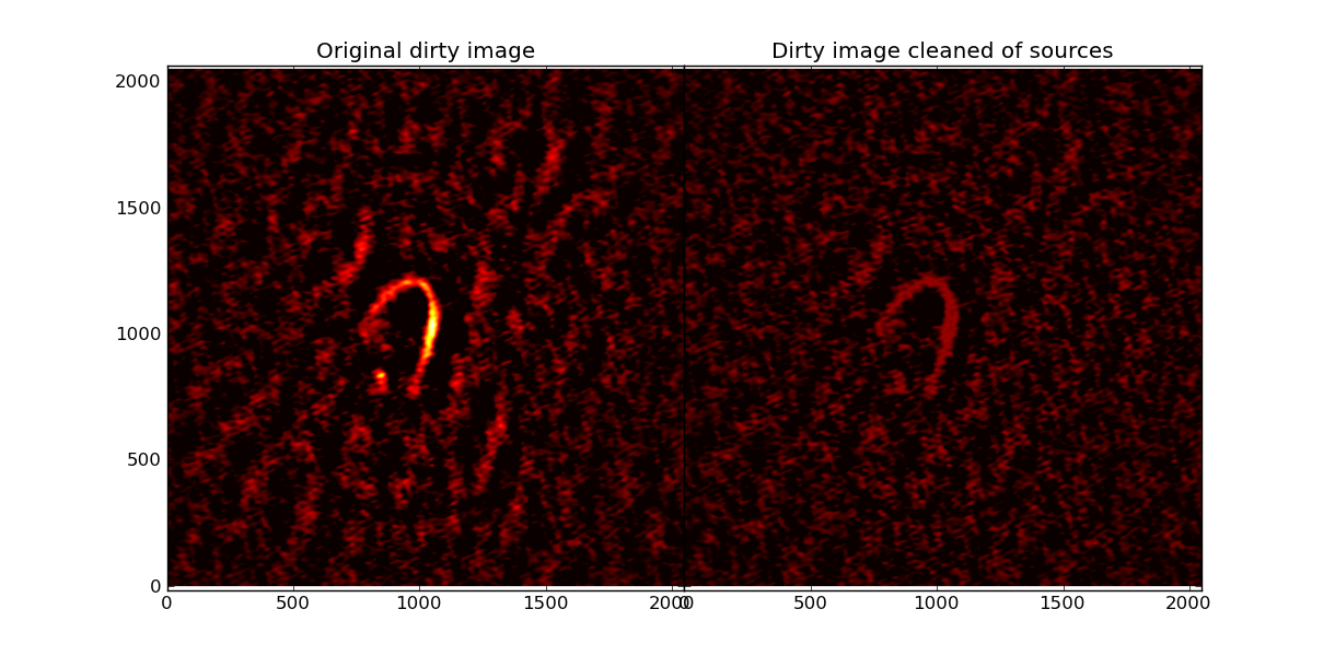
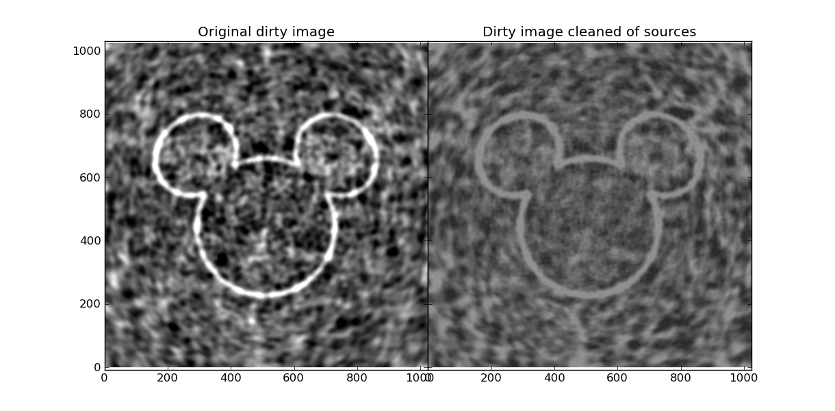
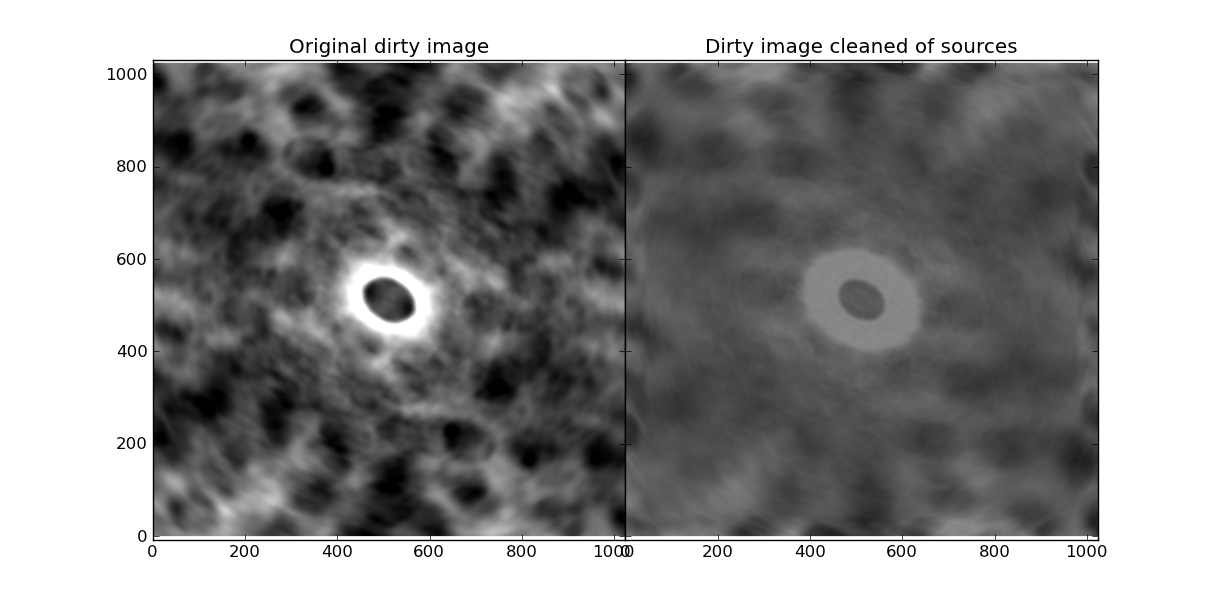
After removing these 2700 “point sources” from the dirty image, the source ϵ Mouse is essentially completely removed (flux is zero, shown as gray below) and the variance in the background, produced by the sidelobes of the dirty beam convolved with the source, is much lower (less negative/positive; more gray).

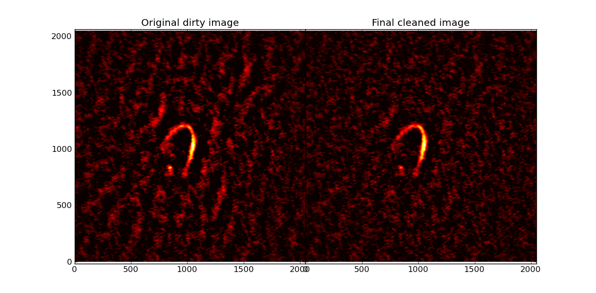
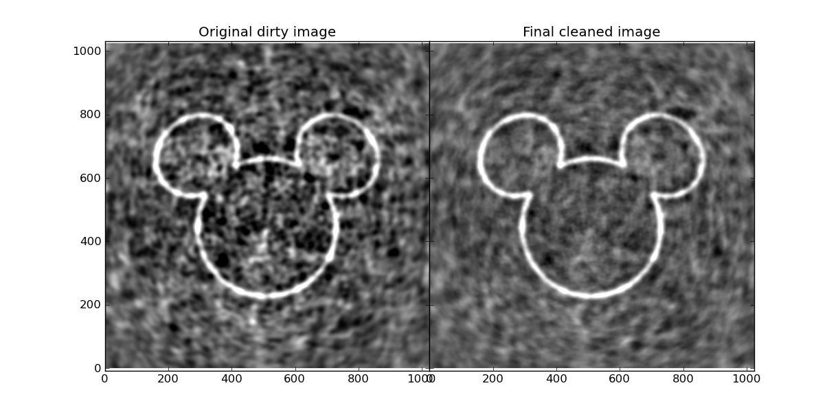
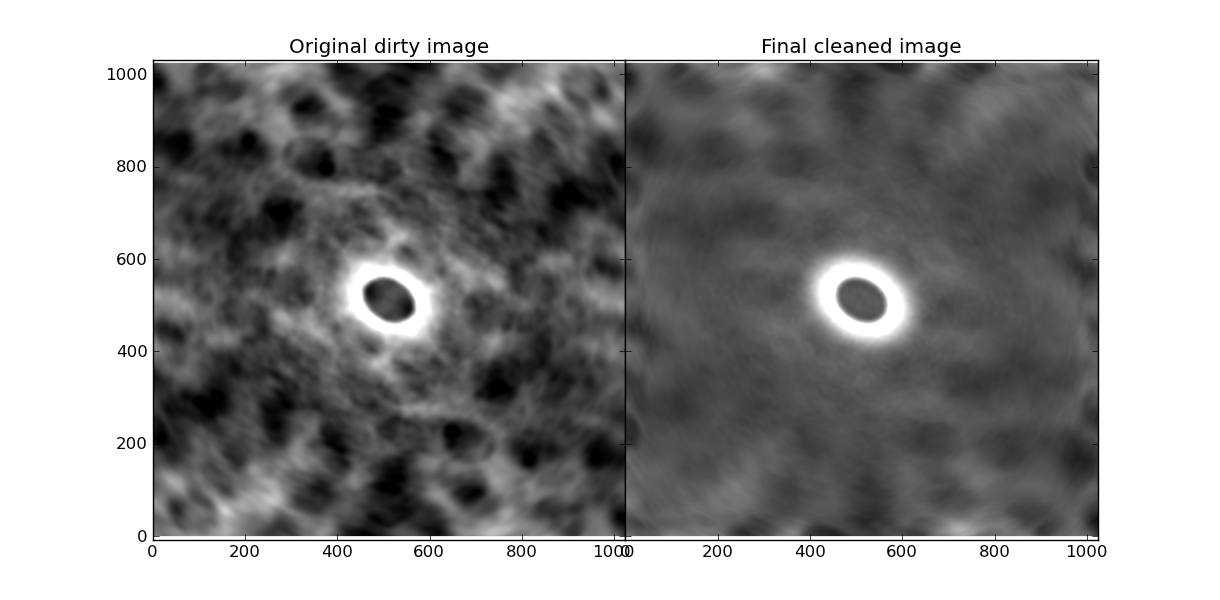
Finally, the remaining background variance is added to the model image, convolved with the clean beam, to produce the final, CLEANed image (right). In this image, the effects of the sidelobes of the dirty beam are largely removed. When compared with the original dirty image (left), the source ϵ Mouse is more clear and the variance in the background is significantly smaller.

As an additional example of a more realistic simulated astrophysical source, we applied our code to a simulated inclined disk, like the protoplanetary disks we find around young stars.

Click on the image below to see an animated version.

This dataset is one of the earliest published science data from the ALMA telescope array and was obtained by Boley et al. (2012). For a great description of this data and the Fomalhaut system, see Astrobites. We thank Aaron Boley and Matt Payne for use of the data.

Click on the image below to see an animated version.